Standard Cartesian coordinates are commonly used to describe points in the plane. If we mention the point \((4,3)\text{,}\) we know that we arrive at this point from the origin by moving four units to the right and three units up.
Sometimes, however, it is more natural to work in a different coordinate system. Suppose that you live in the city whose map is shown in Figure 3.2.1 and that you would like to give a guest directions for getting from your house to the store. You would probably say something like, "Go four blocks up Maple. Then turn left on Main for three blocks." The grid of streets in the city gives a more natural coordinate system than standard north-south, east-west coordinates.
A street map of a fictitious city with two sets of parallel streets and an arrow indicating that north is to the top of the map. One set of streets runs roughly southwest to northeast, and one of these streets is labelled “Maple” and has a marked location labelled “House”. A second set of streets runs roughly northwest to southeast and has a street labelled “Main” with a location labelled “Store”.
In this section, we will develop the concept of a basis through which we will create new coordinate systems in \(\real^m\text{.}\) We will see that the right choice of a coordinate system provides a more natural way to approach some problems.
There is a set of coordinate axes and a standard \(1\times1\) coordinate grid in the background. There are also two vectors \(\vvec_1=\twovec21\) and \(\vvec_2=\twovec12\) and two sets of parallel lines representing the linear combinations of \(\vvec_1\) and \(\vvec_2\text{.}\) One set of parallel lines is parallel to \(\vvec_1\) and passes through the integer multiples of \(\vvec_2\) while the other set is parallel to \(\vvec_2\) and passes through integer multiples of \(\vvec_1\text{.}\)
In the preview activity, we worked with a set of two vectors in \(\real^2\) and found that we could express any vector in \(\real^2\) in two different ways: in the usual way where the components of the vector describe horizontal and vertical changes, and in a new way as a linear combination of \(\vvec_1\) and \(\vvec_2\text{.}\) We could also translate between these two descriptions. This example illustrates the central idea of this section.
In the preview activity, we created a new coordinate system for \(\real^2\) using linear combinations of a set of two vectors. More generally, the following definition will guide us.
A set of vectors \(\vvec_1,\vvec_2,\ldots,\vvec_n\) in \(\real^m\) is called a basis for \(\real^m\) if the set of vectors spans \(\real^m\) and is linearly independent.
If a set of vectors \(\vvec_1,\vvec_2,\ldots,\vvec_n\) forms a basis for \(\real^m\text{,}\) what can you guarantee about the pivot positions of the matrix
We know that the span of the set of vectors is \(\real^m\) if and only if \(A\) has a pivot position in every row. We also know that the set of vectors is linearly independent if and only if \(A\) has a pivot position in every column. This means that a set of vectors forms a basis if and only if \(A\) has a pivot in every row and every column. Therefore, \(A\) must be row equivalent to the identity matrix \(I\text{:}\)
In addition to helping identify bases, this fact tells us something important about the number of vectors in a basis. Since the matrix \(A\) has a pivot position in every row and every column, it must have the same number of rows as columns. Therefore, the number of vectors in a basis for \(\real^m\) must be \(m\text{.}\) For example, a basis for \(\real^{23}\) must have exactly 23 vectors.
form the columns of the \(3\times3\) identity matrix, which implies that this set forms a basis for \(\real^3\text{.}\) More generally, the set of vectors \(\evec_1,\evec_2,\ldots,\evec_m\) forms a basis for \(\real^m\text{,}\) which we call the standard basis for \(\real^m\text{.}\)
A basis for \(\real^m\) forms a coordinate system for \(\real^m\text{,}\) as we will describe. Rather than continuing to write a list of vectors, we will find it convenient to denote a basis using a single symbol, such as
In the standard coordinate system, the point \((2,-3)\) is found by moving 2 units to the right and 3 units down. We would like to define a new coordinate system where we interpret \((2,-3)\) to mean we move two times along \(\vvec_1\) and 3 times along \(-\vvec_2\text{.}\) As we see in the figure, doing so leaves us at the point \((1,-4)\text{,}\) expressed in the usual coordinate system.
There is a set of coordinate axes and a standard \(1\times1\) coordinate grid in the background. There are also two vectors \(\vvec_1=\twovec21\) and \(\vvec_2=\twovec12\) and two sets of parallel lines representing the linear combinations of \(\vvec_1\) and \(\vvec_2\text{.}\) One set of parallel lines is parallel to \(\vvec_1\) and passes through the integer multiples of \(\vvec_2\) while the other set is parallel to \(\vvec_2\) and passes through integer multiples of \(\vvec_1\text{.}\)
The coordinates of the vector \(\xvec\) in the new coordinate system are the weights that we use to create \(\xvec\) as a linear combination of \(\vvec_1\) and \(\vvec_2\text{.}\)
Since we now have two descriptions of the vector \(\xvec\text{,}\) we need some notation to keep track of which coordinate system we are using. Because \(\twovec{1}{-4} = 2\vvec_1 - 3\vvec_2\text{,}\) we will write
More generally, \(\coords{\xvec}{\bcal}\) will denote the coordinates of \(\xvec\) in the basis \(\bcal\text{;}\) that is, \(\coords{\xvec}{\bcal}\) is the vector \(\twovec{c_1}{c_2}\) of weights such that
Suppose we know the expression of a vector \(\xvec\) in standard coordinates. How can we find its coordinates in the basis \(\bcal\text{?}\) For instance, suppose \(\xvec=\twovec{-8}{2}\) and that we would like to find \(\coords{\xvec}{\bcal}\text{.}\) We can write
This example illustrates how a basis in \(\real^2\) provides a new coordinate system for \(\real^2\) and shows how we may translate between this coordinate system and the standard one.
More generally, suppose that \(\bcal=\{\vvec_1,\vvec_2,\ldots,\vvec_m\}\) is a basis for \(\real^m\text{.}\) We know that the span of the vectors is \(\real^m\text{,}\) which implies that any vector \(\xvec\) in \(\real^m\) can be written as a linear combination of the vectors. In addition, we know that the vectors are linearly independent, which means that we can write \(\xvec\) as a linear combination of the vectors in exactly one way. Therefore, we have
Find a matrix \(A\) such that, for any vector \(\xvec\text{,}\) we have \(\xvec = A\coords{\xvec}{\bcal}\text{.}\) Explain why this matrix is invertible.
Using what you found in the previous part, find a matrix \(B\) such that, for any vector \(\xvec\text{,}\) we have \(\coords{\xvec}{\bcal} = B\xvec\text{.}\) What is the relationship between the two matrices \(A\) and \(B\text{?}\) Explain why this relationship holds.
Find a matrix \(C\) that converts coordinates in the basis \(\ccal\) into coordinates in the basis \(\bcal\text{;}\) that is,
\begin{equation*}
\coords{\xvec}{\bcal} = C \coords{\xvec}{\ccal}\text{.}
\end{equation*}
You may wish to think about converting coordinates from the basis \(\ccal\) into the standard coordinate system and then into the basis \(\bcal\text{.}\)
This activity demonstrates how we can efficiently convert between coordinate systems defined by different bases. Let’s consider a basis \(\bcal = \{\vvec_1,\vvec_2,\ldots,\vvec_m\}\) and a vector \(\xvec\text{.}\) We know that
where \(P_{\bcal} = \left[\begin{array}{rrrr}
\vvec_1 \amp \vvec_2 \amp \cdots \amp \vvec_m
\end{array}\right]\text{.}\) This means that the matrix \(P_{\bcal}\) converts coordinates in the basis \(\bcal\) into standard coordinates.
Since the columns of \(P_{\bcal}\) are the basis vectors \(\vvec_1,\vvec_2,\ldots,\vvec_m\text{,}\) we know that \(P_{\bcal}
\sim I_m\text{,}\) and \(P_{\bcal}\) is therefore invertible. Since we have
If we have another basis \(\ccal\text{,}\) we find, in the same way, that \(\xvec = P_{\ccal}\coords{\xvec}{\ccal}\) for the conversion between coordinates in the basis \(\ccal\) into standard coordinates. We then have
It is relatively straightforward to convert a vector’s representation in this basis into to the standard basis using the matrix whose columns are the basis vectors:
For example, suppose that the vector \(\xvec\) is described in the coordinate system defined by the basis as \(\coords{\xvec}{\bcal} = \threevec{2}{-2}{1}\text{.}\) We then have
Consider now the vector \(\xvec=\threevec{3}{1}{-2}\text{.}\) If we would like to express \(\xvec\) in the coordinate system defined by \(\bcal\text{,}\) then we compute
Four data points are plotted representing a company’s revenue in the four quarters of a year. The horizontal axis is labelled “Quarter” and indicates quarters one, two, three, and four. The vertical axis is labelled “Revenue” and has labelled positions five, ten, and fifteen. The data points are plotted at \((1,10.3)\text{,}\)\((2,13.1)\text{,}\)\((3,7.5)\text{,}\) and \((4,8.2)\text{.}\)
In the upper left is a representation of \(\vvec_1\) where each point has a vertical coordinate of one. The upper right shows a representation of \(\vvec_2\text{,}\) whose first two points have a vertical coordinate of one and whose last two points have a vertical coordinate of minus one.
In the lower left is a representation of \(\vvec_3\text{.}\) The vertical coordinates of the points from left to right are one, negative one, zero, and zero. In the lower right, the vertical coordinates are zero, zero, one, and negative one, which represents \(\vvec_4\text{.}\)
This diagram plots the four revenue data points as before and adds a horiztonal line drawn at the average of the four revenue values and extending across the width of the diagram.
The average revenue for the first two quarters is 11.7, which is 1.925 million dollars above the yearly average. Similarly, the average revenue for the last two quarters is 1.925 million dollars below the yearly average. This is recorded by the second term
The four revenue data points are again plotted with a horizontal line indicating the average drawn in the background. There are two horizontal line segments added, the first of which represents the average of the first two quarters with the second representing the average of the last two quarters. The two new horizontal lines show the difference in the averages over the two halves of the year compared to the average over the entire year.
Finally, the first quarter’s revenue is 1.400 million dollars below the average over the first two quarters and the second quarter’s revenue is 1.400 million dollars above that average. This, and the corresponding data for the last two quarters, is captured by the last two terms:
The four revenue data points are plotted with two horizontal lines indicating the averages over the first and second halves of the year drawn in the background.
There are also four new horizontal lines passing through each of the data points that indicate the revenue in each quarter. This demonstrates how the revenue in each quarter differs from the average revenue over its half of the year.
If we write \(\coords{\xvec}{\bcal} =
\fourvec{c_1}{c_2}{c_3}{c_4}\text{,}\) we see that the coefficient \(c_1\) measures the average revenue over the year, \(c_2\) measures the deviation from the annual average in the first and second halves of the year, and \(c_3\) measures how the revenue in the first and second quarter differs from the average in the first half of the year. In this way, the coefficients provide a view of the revenue over different time scales, from an annual summary to a finer view of quarterly behavior.
This basis is sometimes called a Haar wavelet basis, and the change of basis is known as a Haar wavelet transform. In the next section, we will see how this basis provides a useful way to store digital images.
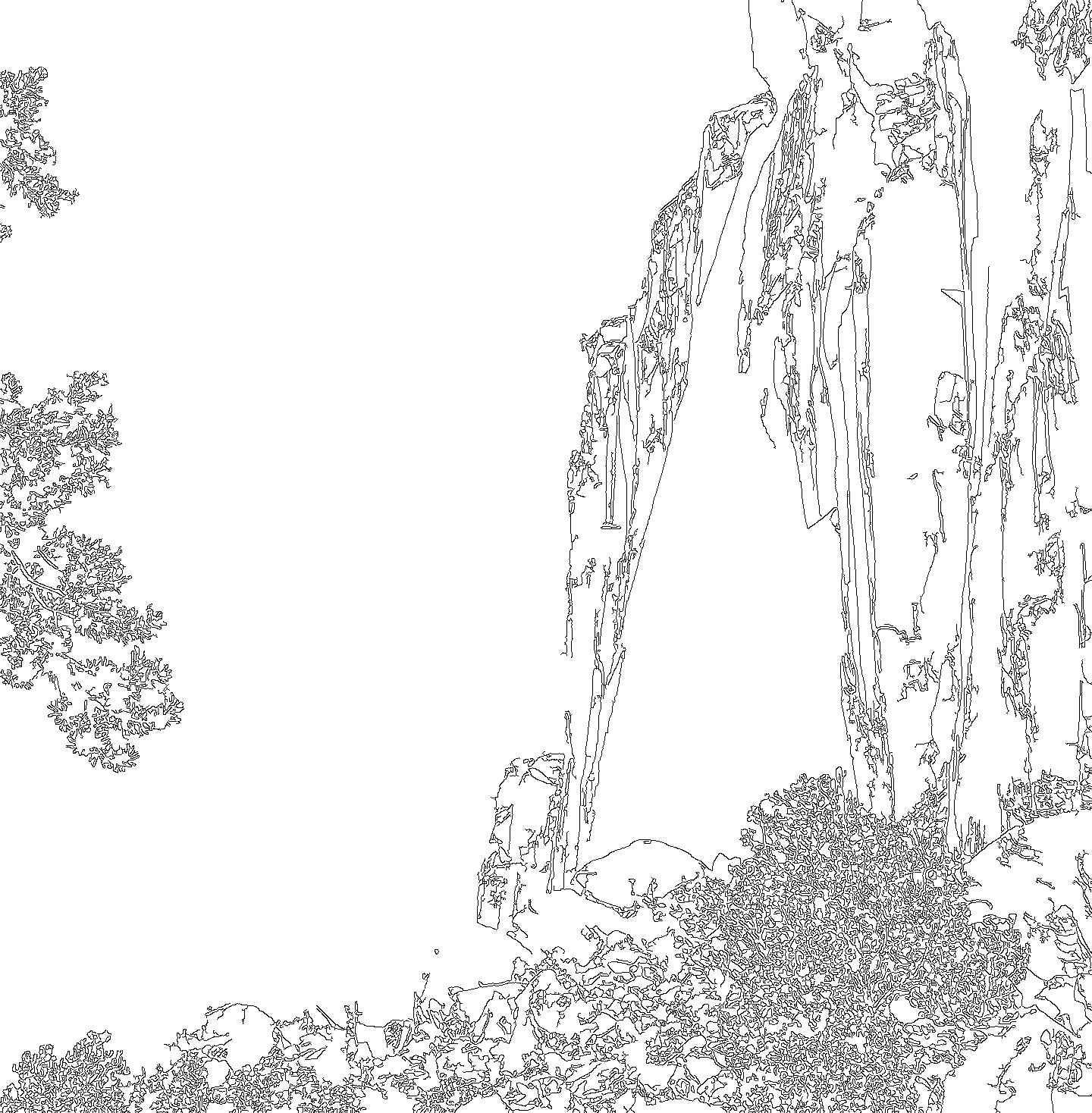
An important problem in the field of computer vision is to detect edges in a digital photograph, as is shown in Figure 3.2.12. Edge detection algorithms are useful when, say, we want a robot to locate an object in its field of view. Graphic designers also use these algorithms to create artistic effects.
A color photograph showing a red rock canyon wall against a blue sky. There are a few shadows in the canyon wall, but the region of the photograph occupied by the wall is fairly homogeneous. The blue sky is also fairly homogeneous so that there is a sharp division between the area occupied by the canyon wall and the area occupied by the sky. There is also some vegetation at the bottom and branches of a tree on the left.
This image has a pure white background and curves drawn in black indicating edges detected in the photograph. There is a prominent vertical curve representing the edge between the canyon wall and the sky. Additional curves highlight some of the shadows in the canyon wall as well as the vegetation and branches of the tree.
We will consider a very simple version of an edge detection algorithm to give a sense of how this works. Rather than considering a two-dimensional photograph, we will think about a one-dimensional row of pixels in a photograph. The grayscale values of a pixel measure the brightness of a pixel; a grayscale value of 0 corresponds to black, and a value of 255 corresponds to white.
A horizontal axis with labelled locations one through six representing the six pixels and a vertical axis with a scale from zero to 250. There are six points plotted representing the grayscale values of the six pixels. The first four grayscale values are relatively small, but the fifth and sixth are relatively large so that we see a jump in the values between the fourth and fifth pixel.
We can easily see that there is a jump in brightness between pixels 4 and 5, but how can we detect it computationally? We will introduce a new basis \(\bcal\) for \(\real^6\) with vectors:
Determine the matrix \(P_\bcal^{-1}\) that converts the representation of \(\xvec\) in standard coordinates into the coordinate system defined by \(\bcal\text{.}\)
Using the relationship \(\coords{\xvec}{\bcal} =
P_{\bcal}^{-1}\xvec\text{,}\) determine an expression for the coefficient \(c_2\) in terms of \(x_1,x_2,\ldots,x_6\text{.}\) What does \(c_2\) measure in terms of the grayscale values of the pixels? What does \(c_4\) measure in terms of the grayscale values of the pixels?
Explain how the coefficients in \(\coords{\xvec}{\bcal}\) determine the location of the jump in brightness in the grayscale values represented by the vector \(\xvec\text{.}\)
Readers who are familiar with calculus may recognize that this change of basis converts a vector \(\xvec\) into \(\coords{\xvec}{\bcal}\text{,}\) the set of changes in \(\xvec\text{.}\) This process is similar to differentiation in calculus. Similarly, the process of converting \(\coords{\xvec}{\bcal}\) into the vector \(\xvec\) adds together the changes in a process similar to integration. As a result, this change of basis represents a linear algebraic version of the Fundamental Theorem of Calculus.
We defined a basis to be a set of vectors \(\bcal =
\{\vvec_1,\vvec_2,\ldots,\vvec_n\}\) that is linearly independent and whose span is \(\real^m\text{.}\)
A set of vectors forms a basis for \(\real^m\) if and only if the matrix
If \(\vvec_1,\vvec_2,\ldots,\vvec_m\) forms a basis for \(\real^m\text{,}\) then any vector in \(\real^m\) can be written as a linear combination of the vectors in exactly one way.
We used the basis \(\bcal\) to define a coordinate system in which \(\coords{\xvec}{\bcal} = \cfourvec{c_1}{c_2}{\vdots}{c_n}
\text{,}\) the coordinates of \(\xvec\) in the basis \(\bcal\text{,}\) are defined by
There is a standard \(1\times1\) coordinate grid and a set of labelled coordinate axes. The vectors \(\vvec_1=\twovec21\) and \(\vvec_2=\twovec{-2}2\) are shown along with the usual sets of lines parallel to both vectors.
Explain how to convert \(\coords{\xvec}{\bcal}\text{,}\) the representation of a vector \(\xvec\) in the coordinates defined by \(\bcal\text{,}\) into \(\xvec\text{,}\) its representation in the standard coordinate system.
Explain how to convert the vector \(\xvec\) into \(\coords{\xvec}{\bcal}\text{,}\) its representation in the coordinate system defined by \(\bcal\text{.}\)
Explain why \(\bcal=\{\vvec_1,\vvec_2,\vvec_3\}\) is a basis for \(\real^3\text{.}\) Notice that you may enter \(\cos\left(\frac\pi6\right)\) into Sage as cos(pi/6).
Find the matrices \(P_{\bcal}\) and \(P_{\bcal}^{-1}\text{.}\) If \(\xvec=\threevec{x_1}{x_2}{x_3}\) and \(\coords{\xvec}{\bcal} = \threevec{c_1}{c_2}{c_3}\text{,}\) explain why \(c_1\) is the average of \(x_1\text{,}\)\(x_2\text{,}\) and \(x_3\text{.}\)
If \(\bcal=\{\vvec_1,\vvec_2,\ldots,\vvec_n\}\) is a basis of \(\real^m\text{,}\) then every vector in \(\real^m\) can be expressed as a linear combination of basis vectors.
Suppose we have an invertible \(m\times m\) matrix \(A\text{,}\) and we perform a sequence of row operations on \(A\) to form a matrix \(B\text{.}\) Can you guarantee that the columns of \(B\) form a basis for \(\real^m\text{?}\)
Suppose you have a set of 10 vectors in \(\real^{10}\) and that every vector in \(\real^{10}\) can be written as a linear combination of these vectors. Can you guarantee that this set of vectors is a basis for \(\real^{10}\text{?}\)
Crystallographers find it convenient to use coordinate systems that are adapted to the specific geometry of a crystal. As a two-dimensional example, consider a layer of graphite in which carbon atoms are arranged in regular hexagons to form the crystalline structure shown in Figure 3.2.14.
A regular hexagonal array of carbon atoms. The top and bottom of each hexagon is horizontal and each edge belongs to two hexagons. Attention is drawn to a special hexagon in which the bottom left carbon atom is denoted \(0\text{.}\) There is a vector \(\vvec_1\) that begins at the carbon atom labelled \(0\) and extends horizontally to the next carbon atom. A second vector \(\vvec_1\) begins at the carbon atom labelled \(0\) and extends upward and to the left to the adjacent carbon atom in that hexagon.
There is another carbon atom denoted by \(1\text{.}\) To travel to this carbon atom from the atom labelled \(0\text{,}\) one walks through a sequence of carbon atoms, first moving horizontally, then upward and to the right, then horizontally, and finally upward and to the right.
The origin of the coordinate system is at the carbon atom labeled by “0”. It is convenient to choose the basis \(\bcal\) defined by the vectors \(\vvec_1\) and \(\vvec_2\) and the coordinate system it defines.
How do the coordinates of the atoms in the hexagon whose lower left corner is labeled “1” compare to the coordinates in the hexagon whose lower left corner is labeled "0"?
You should find that the matrix \(D\) is a very simple matrix, which means that this basis \(\bcal\) is well suited to study the effect of multiplication by \(A\text{.}\) This observation is the central idea of the next chapter.