Matrix transformations, which we explored in the last section, allow us to describe certain functions \(T:\real^n\to\real^m\text{.}\) In this section, we will demonstrate how matrix transformations provide a convenient way to describe geometric operations, such as rotations, reflections, and scalings. We will then explore how matrix transformations are used in computer animation.
We will describe the matrix transformation \(T\) that reflects 2-dimensional vectors across the horizontal axis. For instance, Figure 2.6.1 illustrates how a vector \(\xvec\) is reflected onto the vector \(T(\xvec)\text{.}\)
Use your results to write the matrix \(A\) so that \(T(\xvec) = A\xvec\text{.}\) Then verify that \(T\left(\twovec{x}{y}\right)\) agrees with what you found in part b.
Describe the transformation that results from composing \(T\) with itself; that is, what is the transformation \(T\circ T\text{?}\) Explain how matrix multiplication can be used to justify your response.
Subsection2.6.1The geometry of \(2\times2\) matrix transformations
We have now seen how a few geometric operations, such as rotations and reflections, can be described using matrix transformations. The following activity shows, more generally, that matrix transformations can perform a variety of important geometric operations.
Activity2.6.2.Using matrix transformations to describe geometric operations.
Instructions.
The diagram below demonstrates the effect of a matrix transformation \(T\) on the plane. You may modify the matrix \(A=\begin{bmatrix} a \amp b \\ c \amp c
\\ \end{bmatrix}\) defining \(T\) through the sliders at the top.
Since a matrix transformation takes a vector as input and produces a vector as output, we will show the inputs and outputs on separate sets of axes. In particular, the axes on the left represent the inputs while the axes on the right illustrate how input features are transformed by \(T\text{.}\)
For the following \(2\times2\) matrices \(A\text{,}\) use the diagram to study the effect of the corresponding matrix transformation \(T(\xvec) =
A\xvec\text{.}\) For each transformation, describe the geometric effect the transformation has on the plane.
The previous activity presented some examples showing that matrix transformations can perform interesting geometric operations, such as rotations, scalings, and reflections. Before we go any further, we should explain why it is possible to represent these operations by matrix transformations. In fact, we ask more generally: what types of functions \(T:\real^n\to\real^m\) are represented as matrix transformations?
The linearity of matrix-vector multiplication provides the key to answering this question. Remember that if \(A\) is a matrix, \(\vvec\) and \(\wvec\) vectors, and \(c\) a scalar, then
It turns out that, if \(T:\real^n\to\real^m\) satisfies these two linearity properties, then we can find a matrix \(A\) such that \(T(\xvec) = A\xvec\text{.}\) In fact, Proposition 2.5.6 tells us how to form \(A\text{;}\) we simply write
\begin{equation*}
A = \left[\begin{array}{rrrr}
\end{array}\right]\text{.}
\end{equation*}
We will now check that \(T(\xvec) = A\xvec\) using the linearity of \(T\text{:}\)
Said simply, this proposition means says that if have a function \(T:\real^n\to\real^m\) and can verify the two linearity properties stated in the proposition, then we know that \(T\) is a matrix transformation. Let’s see how this works in practice.
We will consider the function \(T:\real^2\to\real^2\) that rotates a vector \(\xvec\) by \(45^\circ\) in the counterclockwise direction to obtain \(T(\xvec)\) as seen in Figure 2.6.5.
There are two figures shown on the left and on the right. The figure on the left contains the vector \(\xvec=\twovec31\) while the figure on the right has the vector \(T(\xvec)\) obtained by rotating \(\xvec\) counterclockwise by 45 degrees.
We first need to know that \(T\) can be represented by a matrix transformation, which means, by Proposition 2.6.3, that we need to verify the linearity properties:
The next two figures illustrate why these properties hold. For instance, Figure 2.6.6 shows the relationship between \(T(\vvec)\) and \(T(c\vvec)\) when \(c\) is a scalar. In particular, scaling a vector and then rotating it is the same as rotating and then scaling it, which means that \(T(c\vvec)
= cT(\vvec)\text{.}\)
Two figures are shown side by side. On the left is a vector \(\vvec\) and a scalar multiple \(c\vvec\text{,}\) both of which lie on the same line. The matrix transformation \(T\) rotates vectors counterclockwise by 45 degrees. In the figure on the right are the vectors \(T(\vvec)\) and \(T(c\vvec)\text{,}\) which again lie on the same line. This demonstrates that \(T(c\vvec) = cT(\vvec)\text{.}\)
Similarly, Figure 2.6.7 shows the relationship between \(T(\vvec+\wvec)\text{,}\)\(T(\vvec)\text{,}\) and \(T(\wvec)\text{.}\) Remember that the sum of two vectors is represented by the diagonal of the parallelogram defined by the two vectors. The rotation \(T\) has the effect of rotating the parallelogram defined by \(\vvec\) and \(\wvec\) into the parallelogram defined by \(T(\vvec)\) and \(T(\wvec)\text{,}\) explaining why \(T(\vvec+\wvec) = T(\vvec) + T(\wvec)\text{.}\)
Two figures are presented, one on the left and one on the right. In the left figure are the vectors \(\vvec\) and \(\wvec\text{,}\) the parallelogram formed by them, and their vector sum \(\vvec+\wvec\text{.}\) Denoting the transformation that rotates vectors counterclockwise by 45 degrees, the right figure contains the vectors \(T(\vvec)\) and \(T(\wvec)\text{,}\) the parallelogram formed by them, and the vector \(T(\vvec+\wvec)\text{,}\) which forms the diagonal of this parallelogram. This demonstrates that \(T(\vvec+\wvec) = T(\vvec) + T(\wvec)\text{.}\)
Figure2.6.7.We see that the vector \(T(\vvec+\wvec)\) is the sum of \(T(\vvec)\) and \(T(\wvec)\) so that \(T(\vvec + \wvec) = T(\vvec) + T(\wvec)\text{.}\)
Having verified these two properties, we now know that the function \(T\) that rotates vectors by \(45^\circ\) is a matrix transformation. We may therefore write it as \(T(\xvec) = A\xvec\) where \(A\) is the \(2\times2\) matrix \(A=\left[\begin{array}{rr} T(\evec_1) \amp T(\evec_2)
\end{array}\right]\text{.}\) The columns of this matrix, \(T(\evec_1)\) and \(T(\evec_2)\text{,}\) are shown on the right of Figure 2.6.8.
The two vector \(\evec_1=\twovec10\) and \(\evec_2=\twovec01\) are shown on the left. On the right is shown the result of rotating both of these vectors counterclockwise by 45 degrees, which is the effect of the matrix transformation \(T\text{.}\)
Notice that \(T(\evec_1)\) forms an isosceles right triangle, as shown in Figure 2.6.9. Since the length of \(\evec_1\) is 1, the length of \(T(\evec_1)\text{,}\) the hypotenuse of the triangle, is also 1, and by Pythagoras’ theorem, the lengths of its legs are \(1/\sqrt{2}\text{.}\)
The vector \(T(\evec_1)\text{,}\) where \(\evec_1=\twovec10\text{,}\) is represented by an arrow that begins at the origin, has length one, and makes a 45 degree angle with the positive horizontal axis. A right triangle is formed by this vector, the horizontal axis, and a vertical line segment from the tip of the vector to the horizontal axis. The legs of this right triangle each have length \(1/\sqrt{2}\text{.}\)
This leads to \(T(\evec_1) = \twovec{\frac1{\sqrt{2}}}
{\frac1{\sqrt{2}}}\text{.}\) In the same way, we find that \(T(\evec_2) = \twovec{-\frac1{\sqrt{2}}}
{\frac1{\sqrt{2}}}\) so that the matrix \(A\) is
The same kind of thinking applies more generally to show that rotations, reflections, and scalings are matrix transformations. Similarly, we could revisit the functions in Activity 2.5.3 and verify that they are matrix transformations.
In this activity, we seek to describe various matrix transformations by finding the matrix that gives the desired transformation. All of the transformations that we study here have the form \(T:\real^2\to\real^2\text{.}\)
Find the matrix of the transformation that has no effect on vectors; that is, \(T(\xvec) = \xvec\text{.}\)
What is the result of composing the reflection you found in the previous part with itself; that is, what is the effect of reflecting across the line \(y=x\) and then reflecting across this line again? Provide a geometric explanation for your result as well as an algebraic one obtained by multiplying matrices.
Compare the result of rotating by \(90^\circ\) and then reflecting in the line \(y=x\) to the result of first reflecting in \(y=x\) and then rotating \(90^\circ\text{.}\)
Find the matrix that results from composing a \(90^\circ\) rotation with itself four times; that is, if \(T\) is the matrix transformation that rotates vectors by \(90^\circ\text{,}\) find the matrix for \(T\circ T\circ T \circ
T\text{.}\) Explain why your result makes sense geometrically.
Subsection2.6.2Matrix transformations and computer animation
Linear algebra plays a significant role in computer animation. We will now illustrate how matrix transformations and some of the ideas we have developed in this section are used by computer animators to create the illusion of motion in their characters.
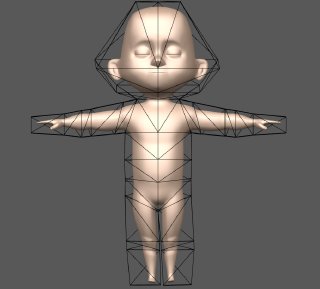
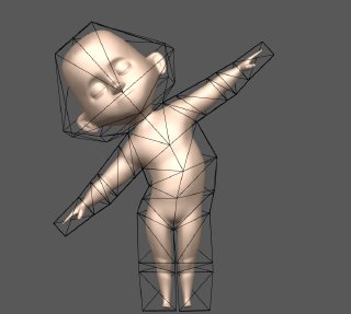
Figure 2.6.10 shows a test character used by Pixar animators. On the left is the original definition of the character; on the right, we see that the character has been moved into a different pose. To make it appear that the character is moving, animators create a sequence of frames in which the character’s pose is modified slightly from one frame to the next often using matrix transformations.
A three dimensional human character used in computer animation. The character is standing upright with both arms extending horizontally to the sides. There is also an set of triangles that form a solid encasing the character. Computer animators move the character by moving the vertices of the triangles.
Of course, realistic characters will be drawn in three-dimensions. To keep things a little more simple, however, we will look at this two-dimensional character and devise matrix transformations that move them into different poses.
A simple two dimensional stick figure that could represent a character in a computer animated film is shown against a coordinate grid and set of axes. The character’s feet are at the points \((-1/2,0)\) and \((1/2,0)\text{.}\) Legs extend from the feet and join the character’s body at \((0,1/2)\text{.}\) The character’s head is an ellipse centered by \((0,2)\) with a vertical span of one unit and a horizontal span of half a unit. The arms are drawn as a single line from \((-1/2,1/2)\) to \((1/2,3/2)\text{.}\)
Of course, the first thing we may wish to do is simply move them to a different position in the plane, such as that shown in Figure 2.6.11. Motions like this are called translations.
This presents a problem because a matrix transformation \(T:\real^2\to\real^2\) has the property that \(T(\zerovec) = A\zerovec = \zerovec\text{.}\) This means that a matrix transformation cannot move the origin of the coordinate plane. To address this restriction, animators use homogeneous coordinates, which are formed by placing the two-dimensional coordinate plane inside \(\real^3\) as the plane \(z=1\text{,}\) as shown in Figure 2.6.12.
A three dimensional diagram with coordinate axes labelled \(x\text{,}\)\(y\text{,}\) and \(z\text{.}\) The two dimensional coordinate plane, including the stick figure character, is included as the plane \(z=1\) so that it appears as a horizontal plane one unit above the origin.
As a result, rather than describing points in the plane as vectors \(\twovec{x}{y}\text{,}\) we describe them as three-dimensional vectors \(\threevec{x}{y}{1}\text{.}\) As we see in the next activity, this allows us to translate our character in the plane.
Since we regard our character as living in \(\real^3\text{,}\) we will consider matrix transformations defined by matrices
\begin{equation*}
\left[\begin{array}{rrr}
a \amp b \amp c \\
d \amp e \amp f \\
0 \amp 0 \amp 1 \\
\end{array}\right]\text{.}
\end{equation*}
Verify that such a matrix transformation transforms points in the plane \(z=1\) into points in the same plane; that is, verify that
\begin{equation*}
\left[\begin{array}{rrr}
a \amp b \amp c \\
d \amp e \amp f \\
0 \amp 0 \amp 1 \\
\end{array}\right]
\threevec{x}{y}{1} = \threevec{x'}{y'}{1}\text{.}
\end{equation*}
Express the coordinates of the resulting point \(x'\) and \(y'\) in terms of the coordinates of the original point \(x\) and \(y\text{.}\)
The diagram below allows you to choose parameters \(a, b, \ldots, f\) to define the matrix associated to the matrix \(\begin{bmatrix}
a \amp b \amp c \\
d \amp e \amp f \\
0 \amp 0 \amp 1 \\
\end{bmatrix}\text{.}\) The transformation’s effect on our character is shown on the right.
As originally drawn, our character is waving with one of their hands. In one of the movie’s scenes, we would like them to wave with their other hand, as shown in Figure 2.6.15. Find the matrix transformation that moves them into this pose.
Later, our character performs a cartwheel by moving through the sequence of poses shown in Figure 2.6.16. Find the matrix transformations that create these poses.
Next, we would like to find the transformations that zoom in on our character’s face, as shown in Figure 2.6.17. To do this, you should think about composing matrix transformations. This can be accomplished in the diagram by using the Compose button, which makes the current pose, displayed on the right, the new beginning pose, displayed on the left. What is the matrix transformation that moves the character from the original pose, shown in the upper left, to the final pose, shown in the lower right?
The the stick figure character has been again translated downward by one unit so that its head is centered at the origin and its feet are half a unit on either side of \((0,-2)\text{.}\)
Starting from the last position, the character has been enlarged by a factor of two. The head is still centered at the origin but the feet are now one unit on either side of \((0,-4)\)
We would also like to create our character’s shadow, shown in the sequence of poses in Figure 2.6.18. Find the sequence of matrix transformations that achieves this. In particular, find the matrix transformation that takes our character from their original pose to their shadow in the lower right.
The character’s feet are still half a horizontal unit on either side of the origin. However, its body forms a 45 degree line from the positive horizontal axis, and its head is centered about the point \((2,2)\text{.}\)
From its previous position, the character has been vertically compressed by a factor of two. The feet are still half a horizontal unit on either side of the origin but the head is now centered on \((2,1)\text{.}\)
From its previous position, the characters has again been vertically compressed by a factor of two. The feet are still half a horizontal unit on either side of the origin but the head is now centered on \((2,1/2)\text{.}\)
For each of the following geometric operations in the plane, find a \(2\times 2\) matrix that defines the matrix transformation performing the operation.
This exercise investigates the composition of reflections in the plane.
Find the result of first reflecting across the line \(y=0\) and then \(y=x\text{.}\) What familiar operation is the cumulative effect of this composition?
What happens if you compose the operations in the opposite order; that is, what happens if you first reflect across \(y=x\) and then \(y=0\text{?}\) What familiar operation results?
It is a general fact that the composition of two reflections results in a rotation through twice the angle from the first line of reflection to the second. We will investigate this more generally in Exercise 2.6.4.8
A set of three dimensional coordinate axes. Each coordinate axis contains a vector of length one pointing in the direction in which the coordinate increases. In particular, we have \(\evec_1=\threevec100\text{,}\)\(\evec_2=\threevec010\text{,}\) and \(\evec_3=\threevec001\text{.}\)
Imagine that the thumb of your right hand points in the direction of \(\evec_1\text{.}\) A positive rotation about the \(x\) axis corresponds to a rotation in the direction in which your fingers point. Find the matrix definining the matrix transformation \(T\) that rotates vectors by \(90^\circ\) around the \(x\)-axis.
What is the cumulative effect of rotating by \(90^\circ\) about the \(x\)-axis, followed by a \(90^\circ\) rotation about the \(y\)-axis, followed by a \(-90^\circ\) rotation about the \(x\)-axis.
If a matrix transformation performs a geometric operation, we would like to find a matrix transformation that undoes that operation.
Suppose that \(T:\real^2\to\real^2\) is the matrix transformation that rotates vectors by \(90^\circ\text{.}\) Find a matrix transformation \(S:\real^2\to\real^2\) that undoes the rotation; that is, \(S\) takes \(T(\xvec)\) back into \(\xvec\) so that \((S\circ T)(\xvec) = \xvec\text{.}\) Think geometrically about what the transformation \(S\) should be and then verify it algebraically.
performs a rotation through an angle \(\theta\) about the origin. Suppose instead that we would like to rotate by \(90^\circ\) about the point \((1,2)\text{.}\) Using homogeneous coordinates, we will develop a matrix that performs this operation.
This is a set of four diagrams. In the upper left is an arrow beginning at the point \((1,2)\text{.}\) In the upper right diagram, the arrow has been translated so that it begins at the origin.
In the lower left, the arrow beginning at the origin has been rotated about the origin. Finally, the diagram in the lower right shows the rotated vector translated back so that it begins at the point \((1,2)\text{.}\)
Consider the matrix transformation \(T:\real^2\to\real^2\) that assigns to a vector \(\xvec\) the closest vector on horizontal axis as illustrated in Figure 2.6.21. This transformation is called the projection onto the horizontal axis. You may imagine \(T(\xvec)\) as the shadow cast by \(\xvec\) from a flashlight far up on the positive \(y\)-axis.
The diagram on the left shows a vector \(\xvec =
\twovec23\text{.}\) The matrix transformation \(T\) projects vertically onto the horizontal axis so that the diagram on the right shows the vector \(T(\xvec) =
\twovec20\text{.}\)
In general, the composition of matrix transformation depends on the order in which we compose them. For these transformations, however, it is not the case. Check this by verifying that
The vector \(\twovec ab\) is represented as an arrow beginning at the origin. The length of the vector is denoted by \(r\) and the angle with the positive horizontal axis by \(\theta\text{.}\)
Suppose we have a matrix transformation \(T\) defined by a matrix \(A\) and another transformation \(S\) defined by \(B\) where
\begin{equation*}
A= \left[\begin{array}{rr}
a \amp -b \\
b \amp a \\
\end{array}\right],~~~
B= \left[\begin{array}{rr}
c \amp -d \\
d \amp c \\
\end{array}\right]\text{.}
\end{equation*}
Describe the geometric effect of the composition \(S\circ
T\) in terms of the \(a\text{,}\)\(b\text{,}\)\(c\text{,}\) and \(d\text{.}\)
We would like to find a similar expression for the matrix that represents the reflection across \(L_\theta\text{,}\) the line passing through the origin and making an angle of \(\theta\) with the positive \(x\)-axis, as shown in Figure 2.6.23.
The line \(L_\theta\) that makes an angle \(\theta\) with the positive horizontal axis along with a vector \(\xvec\text{.}\) The result of reflecting \(\xvec\) in the line \(L_\theta\) is shown and denoted by \(T(\xvec)\text{.}\)
To do this, notice that this reflection can be obtained by composing three separate transformations as shown in Figure 2.6.24. Beginning with the vector \(\xvec\text{,}\) we apply the transformation \(R\) to rotate by \(-\theta\) and obtain \(R(\xvec)\text{.}\) Next, we apply \(S\text{,}\) a reflection in the horizontal axis, followed by \(T\text{,}\) a rotation by \(\theta\text{.}\) We see that \(T(S(R(\xvec)))\) is the same as the reflection of \(\xvec\) in the original line \(L_\theta\text{.}\)
In the upper left diagram is shown a line and a vector \(\xvec\text{.}\) In the upper right is shown the result of rotating the line clockwise so that the line becomes the horizontal axis. The rotated vector is denoted by \(R(\xvec)\text{.}\)
In the lower left, the result of reflecting \(R(\xvec)\) in the horizontal axis is shown and denoted by \(S(R(\xvec))\text{.}\) Finally, in the lower right, the horizontal axis is rotated counterclockwise back into the original line. The resulting vector is now denoted as \(T(S(R(\xvec)))\text{.}\)
Now that we have a matrix that describes the reflection in the line \(L_\theta\text{,}\) show that the composition of the reflection in the horizontal axis followed by the reflection in \(L_\theta\) is a counterclockwise rotation by an angle \(2\theta\text{.}\) We saw some examples of this earlier in Exercise 2.6.4.2.